Once we create the transcript abundance data using Stringtie, we can now perform the differential expression analysis.
With Strigtie, we had created the estimated transcript abundance data which is compatible with Ballgown. The directory structure of the `for_ballgown` directory looks like this:
~/work/rnaseq_ex1$ tree output/for_ballgown/
output/for_ballgown/
├── ERR188044
│   ├── ERR188044_chrX.gtf
│   ├── e2t.ctab
│   ├── e_data.ctab
│   ├── i2t.ctab
│   ├── i_data.ctab
│   └── t_data.ctab
├── ERR188104
│   ├── ERR188104_chrX.gtf
│   ├── e2t.ctab
│   ├── e_data.ctab
│   ├── i2t.ctab
│   ├── i_data.ctab
│   └── t_data.ctab
├── ERR188234
│   ├── ERR188234_chrX.gtf
│   ├── e2t.ctab
│   ├── e_data.ctab
│   ├── i2t.ctab
│   ├── i_data.ctab
│ └── t_data.ctabTo perform the differential gene expression analyis open Rstudio and change working directory to our project directory. Mine was
setwd("//wsl$/Ubuntu/home/<username>/work/rnaseq_ex1")where, <username> was the username in the WSL system.
Import the necessary packages.
library(devtools)
library(ballgown)
library(dplyr)
library(RSkittleBrewer)
library(genefilter)Read phenotype data. The phenotypic data provided in chrX_data/geuvadis_phenodata.csv. It contains sample ids and information about their sex and population.
pheno_data = read.csv("chrX_data/geuvadis_phenodata.csv")
pheno_data ids sex population
1 ERR188044 male YRI
2 ERR188104 male YRI
3 ERR188234 female YRI
4 ERR188245 female GBR
5 ERR188257 male GBR
6 ERR188273 female YRI
7 ERR188337 female GBR
8 ERR188383 male GBR
9 ERR188401 male GBR
10 ERR188428 female GBR
11 ERR188454 male YRI
12 ERR204916 female YRIRead the expression data that was estimated by Stringtie. This will create a ballgown object.
bg_chrX = ballgown(dataDir = "output/for_ballgown", samplePattern = "ERR", pData=pheno_data)
bg_chrXballgown instance with 4183 transcripts and 12 samplesThe bg_chrX is a ballgown object which contains the results to be analyzed using ballgown.
First, we need to filter out the low abundance genes, i.e., genes that have low number of transcripts.
The command texpr(bg_chrX), gets us the transcription data matrix. Each row stands for one transcript and the columns stand for samples. Each value represents the abundance of a transcript in a sample.
Following is how we select only those transcripts which have variance of more than one across samples.
# transcription matrix
transc_mat = texpr(bg_chrX)
# select trancripts with variane > 1
bg = subset(bg_chrX,"rowVars(transc_mat) > 1", genomesubset=TRUE)
bgballgown instance with 2576 transcripts and 12 samplesNote that we do not just want to filter the matrix values but also the corresponding genome-related data as well. The genomesubset=TRUE arguments takes care of this.
So, from 4183 trancripts in our original results, we now have 2576 trancripts.
Plotting the transcript abundance
We can now plot various details about the results.
To plot the transcript from a gene (geneIDs = MSTRG.264)in one particular sample (ERR188044).
plotTranscripts(gene='MSTRG.264',
gown=bg,
samples='ERR188044',
meas='FPKM',
colorby='transcript',
main='transcripts from gene MSTRG.264: sample ERR188044, FPKM')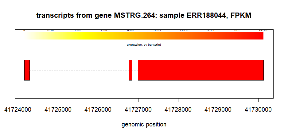
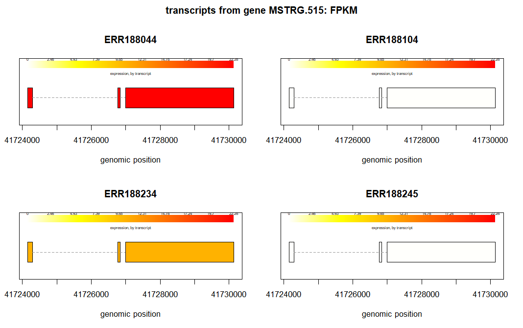
We can also plot the transcript abundance from several samples of same gene. For example, this is an example to plot the transcripts of gene, MSTRG.264, from first four samples from our pheno_data.
plotTranscripts(gene='MSTRG.264',
gown=bg,
samples=pheno_data$ids[1:4],
meas='FPKM',
colorby='transcript',
main='transcripts from gene MSTRG.264: FPKM')
And this is how we plot the mean expression of the gene in different groups, sex in our case here.
plotMeans('MSTRG.264',
bg,
groupvar='sex',
meas='FPKM',
colorby='transcript')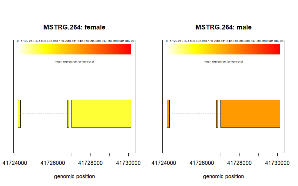
From the above plots we can visualize how the transcript abundance in these genes vary between samples and groups.
Differential expression analysis
Statistical test to identify “transcripts” that show statistically significant differences in expression between
groups. Ballgown uses a parametric F-test comparing nested linear models. Explanation will be written in later posts or can be read from the ballgown paper.
Frazee, Alyssa C., Geo Pertea, Andrew E. Jaffe, Ben Langmead, Steven L. Salzberg, and Jeffrey T. Leek. “Flexible isoform-level differential expression analysis with Ballgown.” Biorxiv (2014): 003665.
results_transcripts = stattest(bg,
feature="transcript",
covariate="sex",
adjustvars = c("population"),
getFC=TRUE,
meas="FPKM")Here,
bgis the ballgown objectfeature="transcript"defines that we are comparing the transcript abundances for differential expression.covariate="sex", means that the differential expression between sexes will be tested. Thesexis a column in ourpdata, i.e. thepheno_dataabove.adjustvars = c("population")tells ballgown to includepopulationas a confounding factor in the test. This also is a column name in thepdata.getFC=TRUEasks the function to estimate and return the fold chang values beteen the two groups (sexin our case).meas="FPKM"selects the FPKM values as selection metric. FPKM stands for Fragments Per Kilobase of transcript per Million mapped reads.
The results_transcripts is a dataframe. Before seeing how these results look like we will add the gene names and ids to it.
results_transcripts = data.frame(geneNames=ballgown::geneNames(bg), geneIDs=ballgown::geneIDs(bg), results_transcripts)
head(results_transcripts) geneNames geneIDs feature id fc pval qval
1 . MSTRG.2 transcript 1 1.4076287 0.4249356 0.7940481
2 PLCXD1 MSTRG.4 transcript 2 0.6628665 0.7588216 0.9265476
3 . MSTRG.4 transcript 3 0.4903795 0.4418855 0.7940481
4 . MSTRG.4 transcript 4 0.6244395 0.7492658 0.9236399
5 . MSTRG.4 transcript 5 1.4556187 0.6647692 0.9027919
6 . MSTRG.5 transcript 6 1.5596317 0.5225704 0.8319786The fc column in the dataframe has the fold change values. The covariate, “sex”, is converted into a factor. In our data we have two sexes, female and male in alphabetical order. So, a value of 1.4 in fc column means that the ratio of expression of the transcript in male /female is 1.4.
In the figure above for geneID, MSTRG.264, we see that the mean expression is higher in male samples. We can verify this is the fc column of the results_transcripts. The value of fc should be greater than 1.
results_transcripts[results_transcripts$geneIDs == 'MSTRG.264', ] geneNames geneIDs feature id fc pval qval
948 GPR82 MSTRG.264 transcript 948 2.263725 0.3370538 0.7940481We can sort the results from smallest p-value to the largest.
results_transcripts = arrange(results_transcripts, pval)This result can be exported to a csv file.
write.csv(results_transcripts, "output/chrX_transcript_results.csv", row.names=FALSE)Draw heatmap
We need to install pheatmap library to plot the heatmap of differentially expressed genes easily.
install.packages("pheatmap")We will start from repeating some of the steps above for clarity.
# read phenotype data (metadata)
pheno_data = read.csv("chrX_data/geuvadis_phenodata.csv")
pheno_data
# read the stringtie results to make ballgown object
bg_chrX <- ballgown(dataDir = "output/for_ballgown",
samplePattern = "ERR",
pData=pheno_data)
class(bg_chrX)
# select transcripts with variance > 1
bg = subset(bg_chrX,"rowVars(transc_mat) >= 1", genomesubset=TRUE)
Perform stattest to get the fold-change data. This time, instead of transcripts, we will apply the stattest to genes.
results_genes = stattest(bg,
                         feature="gene",
                         covariate="sex",
                         adjustvars = c("population"),
                         getFC=TRUE,
                         meas="FPKM")
dim(results_genes) [1] 848 5We have 848 genes. Now, select genes that are significantly differentially expressed.
sig_genes <- subset(results_genes, qval < 0.05)
dim(sig_genes)[1] 4 5So, out of 848 genes only 4 genes have expression that is significantly different between males and females. Note that we have assembled genes present on only X-chromosome so there are only 848 genes our data.
Get the gene expression data in matrix form
# gene expression data
gene_expr <- gexpr(bg)This too will have 848 genes. It will have 12 columns for 12 samples. Check using dim(gene_expr) statement.
Using the sig_genes, we extract expression values of significant genes.
# select significant expr values from sig_gene
sig_gene_expr <- gene_expr[sig_genes$id,]
dim(sig_gene_expr)[1] 4 12head(sig_gene_expr) FPKM.ERR188044 FPKM.ERR188104 FPKM.ERR188234 FPKM.ERR188245
MSTRG.377 462.05763 357.4862 649.32980 548.34972
MSTRG.514 0.00000 0.0000 24.63235 26.10552
MSTRG.515 0.00000 0.0000 291.00042 328.75066
MSTRG.54 66.60243 62.7843 116.19749 94.69623
FPKM.ERR188257 FPKM.ERR188273 FPKM.ERR188337 FPKM.ERR188383
MSTRG.377 321.62584 671.5620 620.18635 282.20474
MSTRG.514 0.00000 0.0000 43.91696 0.00000
MSTRG.515 0.00000 371.1772 900.65095 0.00000
MSTRG.54 61.80819 139.6973 106.17342 66.39131
FPKM.ERR188401 FPKM.ERR188428 FPKM.ERR188454 FPKM.ERR204916
MSTRG.377 359.45425 554.36252 357.81565 645.31369
MSTRG.514 0.00000 9.39225 0.00000 14.39937
MSTRG.515 0.00000 378.61421 0.00000 477.67603
MSTRG.54 79.97481 105.23510 62.06004 111.56535Now we will calculate mean expression of each gene in sig_gene_expr in males and females separately.
From the metadata, we know which columns represent which sex. So, we first make a list of those.
male_cols <- c("FPKM.ERR188044",
               "FPKM.ERR188104",
               "FPKM.ERR188257",
               "FPKM.ERR188383",
               "FPKM.ERR188401",
               "FPKM.ERR188454")

female_cols <- c("FPKM.ERR188234",
                 "FPKM.ERR188245",
                 "FPKM.ERR188273",
                 "FPKM.ERR188337",
                 "FPKM.ERR188428",
"FPKM.ERR204916")Then we create our dataframe for average expression of genes.
sig_avg <- data.frame(
  'male' = rowMeans(sig_gene_expr[, male_cols]),
  'female' = rowMeans(sig_gene_expr[, female_cols])
)
head(sig_avg) male female
MSTRG.377 356.77404 614.85068
MSTRG.514 0.00000 19.74108
MSTRG.515 0.00000 457.97824
MSTRG.54 66.60351 112.26081Some number can be too large, so we will take log2 of the values.
# log2
log_sig_avg <- log2(sig_avg + 1)
head(log_sig_avg) male female
MSTRG.377 8.482905 9.266437
MSTRG.514 0.000000 4.374419
MSTRG.515 0.000000 8.842282
MSTRG.54 6.079026 6.823505The pheatmap requires the data to be a matrix. So, convert the data to a matrix and then plot.
mat_log <- as.matrix(log_sig_avg)
head(mat_log)

pheatmap(
  mat_log,
  cluster_rows = TRUE,         # cluster genes
  cluster_cols = TRUE,         # cluster male/female
  show_rownames = TRUE,        # show gene/transcript names
  show_colnames = TRUE,        # show male/female labels
  color = colorRampPalette(c("blue", "white", "firebrick3"))(100),
  main = "Heatmap of Significant Genes"
)
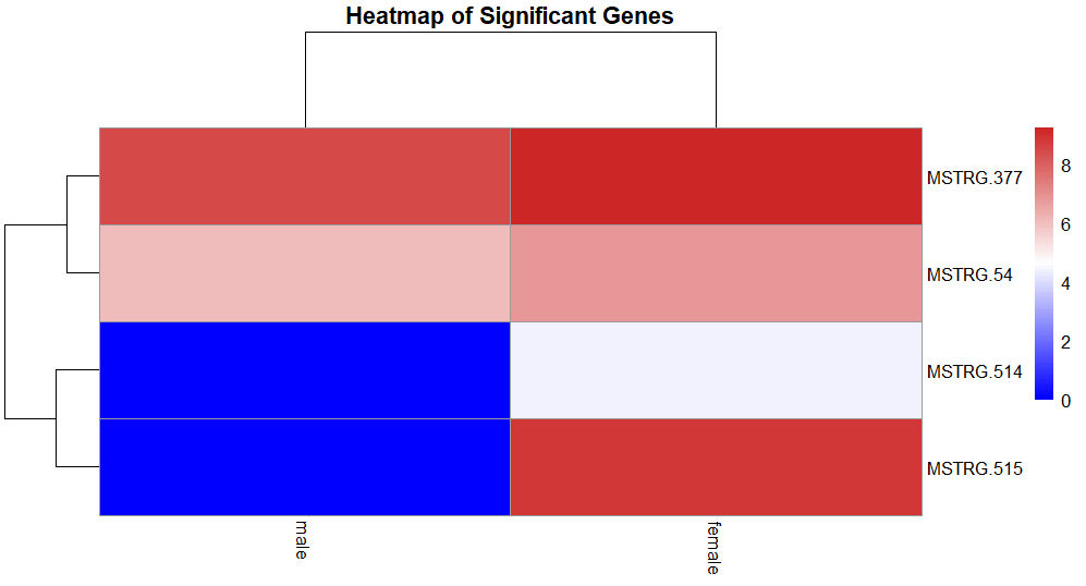
We get the heatmap. We can see that all the genes which are significantly different expression, have higher expression in females.