The deep learning model has model weights which start from a random state wen the model object is created. As we expose the model with the training data, the weights are modified such that their mathematical operations produce values close to the training labels.
Following are the major things that happen during training:
- Weight initialization
- Forward pass of the data through the model layers
- Calculation of loss between output of forward pass and the labels using a loss function.
- Calculation of the gradients with automatic differentiation
- Updating the weights
- Repeat from forward pass.
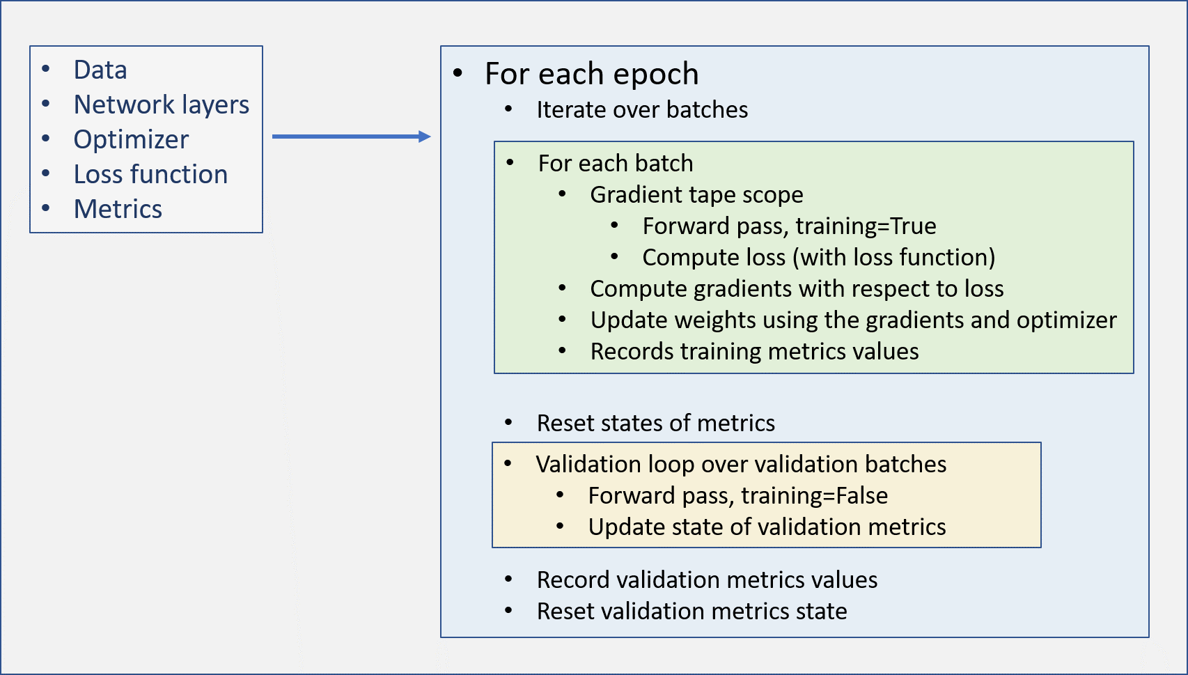
If we want to control exactly how the training occurs, we need to do the training using custom loop for each epoch and batch of the training data, implementing the above steps.
In the custom epoch, each batch of data is passed through the model inside a GradientTape scope. Tensorflow’s GradientTape is used to record the automatic differentiation. Then, the loss is calculated using the loss function.
The GradientTape calculates the gradients of the weights of the model which are then updated using the optimizer.
Following diagram shows the workflow of a custom training loop.
Let’s demonstrate this with an example.
We will take the mnist data, which has 10 classes. We select only three classes from the data and make a multiclass classification model for classifying the data into these three classes. We will select the classes, 0, 1, and 2.
First we will import the python libraries we will need.
import numpy as np
import matplotlib.pyplot as plt

import tensorflow as tf
from tensorflow import keras

from sklearn.utils import shuffleRead data and preprocess
We will use the mnist dataset provided in keras for this tutorial.
We need to know the size and shape of the data. Also, to normalize the data we will see the range of values in the data.
(x_train, y_train), (x_test, y_test) = keras.datasets.mnist.load_data()

x_train, y_train = shuffle(x_train, y_train)

print('\n\nData shape', x_train.shape)
print('minimum', np.min(x_train))
print('maximum', np.max(x_train))Data shape (60000, 28, 28)
minimum 0
maximum 255In this example, we will use only the x_train data to make training and validation datasets. The testing part of the process will not be shown as it is same seen previously.
We see the data values range from 0 to 255. We will divide all the values by 255, to transform the data into numbers in range 0 to 1. This normalization method is sufficient for our data. To normalize other datasets, different nonrmalization methods would be more apporopriate.
x_train = x_train / 255For this example we need each sample to be a flattened array as we will only be using dense layers in neural network. We will see the shape of the data first.
print(x_train[0].shape)(28, 28)So, the samples in the data are shaped (28,28). To flatten the samples, we do the following:
x_train = x_train.reshape(-1, 28*28)
x_train.shape(60000, 784)We will use the first 50,000 samples as training data and the rest as validation data. Remember that we have shuffled the data earlier, so we can use this method to separate the training and validation data.
n_train = 50000
train_data = x_train[:n_train]
train_labels = y_train[:n_train]

val_data = x_train[n_train:]
val_labels = y_train[n_train:]

print(f'{train_data.shape=}')
print(f'{train_labels.shape=}')
print(f'{val_data.shape=}')
print(f'{val_labels.shape=}')train_data.shape=(50000, 784)
train_labels.shape=(50000,)
val_data.shape=(10000, 784)
val_labels.shape=(10000,)Tensorflow dataset and BatchDataset
In the earlier posts we reshaped our data and labels so that it is compatible with the neural network. We reshaped the labels to (numsamples, 1) shape, and the samples to (numsamples, numfeatures, 1).
Here, we will use another method. We will convert our NumPy arrays into tensorflow datasets. Further, we also would make BatchDataset from these datasets using the batch_size. For this example, we will use 32 as the batch size.
For creating the tensorflow dataset, from_tensor_slices method is used. It takes a single argument, a tuple of data and labels.
The batch method of the dataset is used to create batches.
# batch size
batch_size = 32

# prepare training dataset
train_dataset = tf.data.Dataset.from_tensor_slices((train_data, train_labels))
train_dataset = train_dataset.batch(batch_size) # batch dataset

# prepare validation dataset
val_dataset = tf.data.Dataset.from_tensor_slices((val_data, val_labels))
val_dataset = val_dataset.batch(batch_size) # batch datasetGet model
We will make a get_model function to get the neural network. Note that, we will not compile the model as we are going to run a custom loop with GradientTape.
The output layer of the model will have 3 neurons, the same number of classes we have selected. Also, there is no activation function applied to the output layer.
# get model
def get_model():
    # input layer
    inp = keras.layers.Input(shape=train_data.shape[1:])

    # dense layer
    x = keras.layers.Dense(512, activation='relu')(inp)
    x = keras.layers.Dense(256, activation='relu')(x)
    x = keras.layers.Dense(128, activation='relu')(x)

    # output layer
    out =  keras.layers.Dense(10)(x)

    # construct model
    model = keras.Model(inputs=inp, outputs=out)

    return model

model = get_model()Optimizer and loss function
We will use Adam as the optimizer with learning rate 0.001.
For loss function we will use SparseCategoricalCrossentropy as we have three classes and we will not be using the OneHot encoded labels.
# optimizer
optimizer = tf.keras.optimizers.Adam(learning_rate=1e-4)

# loss function
loss_fn = tf.keras.losses.SparseCategoricalCrossentropy(from_logits=True)We will track Accuracy metric.
# metrics
train_acc = keras.metrics.Accuracy()
val_acc = keras.metrics.Accuracy()At the end of each epoch, we will store the loss and accuracy values in a dictionary.
history = {
    'train_loss' : [],
    'val_loss' : [],
    'train_accuracy' : [],
    'val_accuracy' : []
}Training
We now have all the things ready for training our model. We will train the model for 10 epochs.
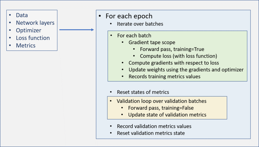
Following is how we implement the training steps as shown in the figure above.
# number of epochs
num_epochs = 10

# iterate over epochs
for ep in range(num_epochs):
  print(f'Epoch {ep+1}')

  # iterate over batches
  for i, (train_batch_data, train_batch_labels) in enumerate(train_dataset):
    # gradient tape
    with tf.GradientTape() as tape:
      logits = model(train_batch_data, training=True)
      loss = loss_fn(train_batch_labels, logits)

    # calculate gradients
    grads = tape.gradient(loss, model.trainable_weights)

    # apply gradients
    optimizer.apply_gradients(zip(grads, model.trainable_weights))

    # update training metric
    preds = tf.argmax(logits, axis=1)
    train_acc.update_state(train_batch_labels, preds)

    # print metric value after every 300 batches
    if i % 300 == 0:
      print(f'Loss = {loss}, Accuracy = {train_acc.result()}')

    # --- batch loop ends here ---------

  # record train loss
  history['train_loss'].append(loss)

  # record training accuracy
  history['train_accuracy'].append(train_acc.result())

  # reset metric state
  train_acc.reset_state()

  # validation loop
  for val_batch_data, val_batch_labels in val_dataset:
    val_logits = model(val_batch_data, training=False)
    val_loss = loss_fn(val_batch_labels, val_logits)

    # update validation metric
    val_preds =  tf.argmax(val_logits, axis=1)
    val_acc.update_state(val_batch_labels, val_preds)

  # record validation loss
  history['val_loss'].append(val_loss)

  # print and record validation accuracy
  print('Validation accuracy: ', val_acc.result())
  history['val_accuracy'].append(val_acc.result())

  # reset states of validation accuracy
  val_acc.reset_state()

# --- epoch loop ends here ---------Epoch 1
Loss = 2.3693222999572754, Accuracy = 0.09375
Loss = 0.3300689458847046, Accuracy = 0.7864410281181335
Loss = 0.22833402454853058, Accuracy = 0.8482736945152283
Loss = 0.48036694526672363, Accuracy = 0.8740982413291931
Loss = 0.0692846029996872, Accuracy = 0.890169620513916
Loss = 0.06315110623836517, Accuracy = 0.9006704092025757
Validation accuracy: tf.Tensor(0.9471, shape=(), dtype=float32)
Epoch 2
Loss = 0.6598396301269531, Accuracy = 0.875
Loss = 0.09225505590438843, Accuracy = 0.9491279125213623
Loss = 0.18820396065711975, Accuracy = 0.9515390992164612
Loss = 0.34771081805229187, Accuracy = 0.9537666440010071
Loss = 0.028796473518013954, Accuracy = 0.9557400345802307
Loss = 0.026022296398878098, Accuracy = 0.9572992920875549
Validation accuracy: tf.Tensor(0.9612, shape=(), dtype=float32)
Epoch 3
Loss = 0.48503226041793823, Accuracy = 0.875
Loss = 0.04891586676239967, Accuracy = 0.9652200937271118
Loss = 0.1606135368347168, Accuracy = 0.9663061499595642
Loss = 0.24057382345199585, Accuracy = 0.9676747918128967
Loss = 0.015865761786699295, Accuracy = 0.9690882563591003
Loss = 0.01238587312400341, Accuracy = 0.9699575304985046
Validation accuracy: tf.Tensor(0.967, shape=(), dtype=float32)
Epoch 4
Loss = 0.28929534554481506, Accuracy = 0.875
Loss = 0.043264687061309814, Accuracy = 0.9738371968269348
Loss = 0.1447778344154358, Accuracy = 0.9750936031341553
Loss = 0.15062391757965088, Accuracy = 0.9758254885673523
Loss = 0.008953276090323925, Accuracy = 0.9770764112472534
Loss = 0.005596090108156204, Accuracy = 0.9779521822929382
Validation accuracy: tf.Tensor(0.9705, shape=(), dtype=float32)
Epoch 5
Loss = 0.1715865135192871, Accuracy = 0.90625
Loss = 0.04048454761505127, Accuracy = 0.9822466969490051
Loss = 0.14332400262355804, Accuracy = 0.9823211431503296
Loss = 0.11258415132761002, Accuracy = 0.9826234579086304
Loss = 0.005552412010729313, Accuracy = 0.9832951426506042
Loss = 0.0025558266788721085, Accuracy = 0.9839690327644348
Validation accuracy: tf.Tensor(0.9726, shape=(), dtype=float32)
Epoch 6
Loss = 0.12078477442264557, Accuracy = 0.9375
Loss = 0.03734421730041504, Accuracy = 0.9870223999023438
Loss = 0.1515222042798996, Accuracy = 0.9867408275604248
Loss = 0.0950898602604866, Accuracy = 0.9872016906738281
Loss = 0.003616809379309416, Accuracy = 0.9876665472984314
Loss = 0.0012269732542335987, Accuracy = 0.9882161617279053
Validation accuracy: tf.Tensor(0.974, shape=(), dtype=float32)
Epoch 7
Loss = 0.08778789639472961, Accuracy = 0.96875
Loss = 0.029765240848064423, Accuracy = 0.9908638000488281
Loss = 0.1529184728860855, Accuracy = 0.990432620048523
Loss = 0.08670826256275177, Accuracy = 0.9909822344779968
Loss = 0.002418466378003359, Accuracy = 0.9912573099136353
Loss = 0.0005564287421293557, Accuracy = 0.9914640188217163
Validation accuracy: tf.Tensor(0.974, shape=(), dtype=float32)
Epoch 8
Loss = 0.05686352401971817, Accuracy = 0.96875
Loss = 0.022822609171271324, Accuracy = 0.9948089718818665
Loss = 0.1572648286819458, Accuracy = 0.9937084317207336
Loss = 0.06381712108850479, Accuracy = 0.9936875700950623
Loss = 0.001745270099490881, Accuracy = 0.9940414428710938
Loss = 0.00030787079595029354, Accuracy = 0.9942746758460999
Validation accuracy: tf.Tensor(0.9756, shape=(), dtype=float32)
Epoch 9
Loss = 0.030033979564905167, Accuracy = 1.0
Loss = 0.023136965930461884, Accuracy = 0.9969891905784607
Loss = 0.1436910629272461, Accuracy = 0.9962042570114136
Loss = 0.03852612525224686, Accuracy = 0.9961154460906982
Loss = 0.001674670958891511, Accuracy = 0.9962010979652405
Loss = 0.00017247656069230288, Accuracy = 0.9962733387947083
Validation accuracy: tf.Tensor(0.976, shape=(), dtype=float32)
Epoch 10
Loss = 0.01602054387331009, Accuracy = 1.0
Loss = 0.018718460574746132, Accuracy = 0.9980273842811584
Loss = 0.1131332591176033, Accuracy = 0.9969841837882996
Loss = 0.0441979318857193, Accuracy = 0.9970518946647644
Loss = 0.0009350811596959829, Accuracy = 0.9968776106834412
Loss = 0.0001424634683644399, Accuracy = 0.9969812035560608
Validation accuracy: tf.Tensor(0.9763, shape=(), dtype=float32)Explanation of the training loop
First we iterate over the epochs and then over the batches with nested for loops.
# number of epochs
num_epochs = 10

# iterate over epochs
for ep in range(num_epochs):
  print(f'Epoch {ep+1}')

  # iterate over batches
for i, (train_batch_data, train_batch_labels) in enumerate(train_dataset):Now, inside a GradientTape scope, we calculate the logits and loss.
with tf.GradientTape() as tape:
  logits = model(train_batch_data, training=True)
loss = loss_fn(train_batch_labels, logits)The logits are raw outputs of the forward pass of the data through the model. The logits have shape (batch_size, output layer size), which in this case is (32, 10).
The training=True sets the model into training mode. In practice, if we have layers such as dropout and BatchNormalization layers, they will behave differently in training and evaluation mode.
The loss is a tensor of type float.
# calculate gradients
grads = tape.gradient(loss, model.trainable_weights)

# apply gradients
optimizer.apply_gradients(zip(grads, model.trainable_weights))The grads are calculated for each batch and the weights updated accordingly.
# update training metric
preds = tf.argmax(logits, axis=1)
train_acc.update_state(train_batch_labels, preds)Update our metric, i.e. train_acc, for each batch. We first get the predictions from the logits. The logits have 10 value for each sample, representing probability of samples belonging to the ten classes. Class with highest probability is the predicted class. This is identified using tf.argmax(logits, axis=1).
# print metric value after every 300 batches
if i % 300 == 0:
print(f'Loss = {loss}, Accuracy = {train_acc.result()}')After every 300 batches, prints out the loss and training accuracy values.
# record train loss
history['train_loss'].append(loss)

# record training accuracy
history['train_accuracy'].append(train_acc.result())Record the values of training loss and training accuracy to the history dictionary.
# reset metric state
train_acc.reset_state()Resets the state of the training accuracy.
# validation loop
for val_batch_data, val_batch_labels in val_dataset:
  val_logits = model(val_batch_data, training=False)
  val_loss = loss_fn(val_batch_labels, val_logits)

  # update validation metric
  val_preds =  tf.argmax(val_logits, axis=1)
val_acc.update_state(val_batch_labels, val_preds)The validation loop passes the validation data through model and outputs the predicted values based on the optimized weights of the model after training. Here we put the model in evaluation mode by setting training=False.
The actual predicted class is calculated using the tf.argmax method.
The loss and accuracy of validation data are recorded in the history dictionary.
# record validation loss
  history['val_loss'].append(val_loss)

  # print and record validation accuracy
  print('Validation accuracy: ', val_acc.result())
history['val_accuracy'].append(val_acc.result())In the end we compile all the results and print the validation accuracy after each epoch.
 # reset states of validation accuracy
val_acc.reset_state()Before the next epoch starts, we reset the state of validation accuracy.
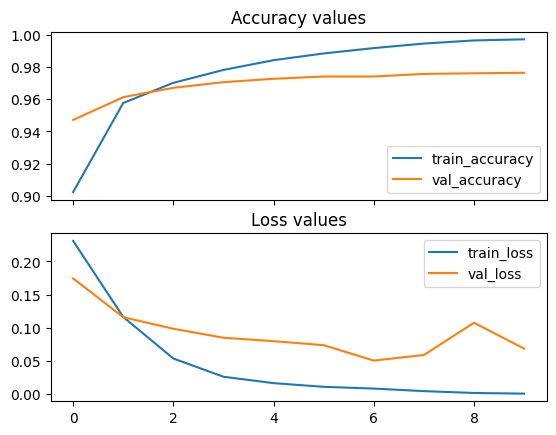
Visualizing the training metrics.
We had stored the loss and accuracy values in the history, which can be plotted using Matplotlib as below.
# plt history
fig , ax = plt.subplots(2, sharex=True)
# accuracy history
ax[0].plot(history['train_accuracy'], label='train_accuracy')
ax[0].plot(history['val_accuracy'], label='val_accuracy')
ax[0].legend()
ax[0].set_title('Accuracy values')


# loss history
ax[1].plot(history['train_loss'], label='train_loss')
ax[1].plot(history['val_loss'], label='val_loss')
ax[1].legend()
ax[1].set_title('Loss values')

plt.show()